
Make Font Red If It Meets a Condition - Without Conditional Formatting
September 12, 2014 - by Bill Jelen
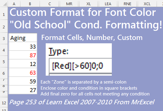
Before there was conditional formatting, there was custom number formatting. You can still add a condition to your custom number formats.
- Select the range of cells. Press Ctrl + 1 to open the Format Cells dialog.
- Select the Number tab. Choose Custom from the bottom of the list.
-
In the Type box, enter a format such as
[Red][>=90];[Blue][>=60]0;0
You can only specify two conditions, so a total of three colors, counting the final ;0 which will show the assigned font color for the cell.
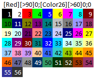
You can only use certain color names… think back to the 3-bit color days: Blue, Black, Yellow, Teal, Red, White. But the little-known secret is you can use any of Excel 2003’s colors with [Color1] through [Color56]. For those of you who never memorized them, here they are:
This is one of the tips in Learn Excel 2007-2010 from MrExcel – 512 Excel Mysteries Solved.