Freeman2022
New Member
- Joined
- Nov 3, 2021
- Messages
- 41
- Office Version
- 365
- Platform
- Windows
Hello,
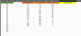
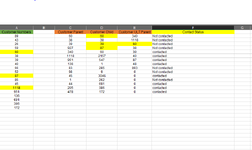
I have a list of numbers in column A listed as Customer numbers, also in columns C,D,E are customer numbers. What I'm trying to do is if Column A info is found in column C,D or E, then Column F is Contacted, if not then not contacted.
Thanks in advance
I'm using excel 365
I have a list of numbers in column A listed as Customer numbers, also in columns C,D,E are customer numbers. What I'm trying to do is if Column A info is found in column C,D or E, then Column F is Contacted, if not then not contacted.
Thanks in advance
I'm using excel 365