How to setup macro to reformat data

[jakeman]

Hi there - I'm not sure how to go about this problem. I have an existing table of data that is in a format which is not very usable. I want to reformat the data in a manner that requires a little bit of coding, otherwise I'll need to do data entry and that will take a long time.

Currently my data is in this format:





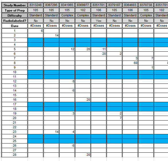
However, I want to have the information in this format instead:



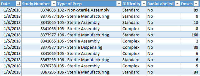
I am trying to create a macro that will step through each Study Number and as many entries there are for a month, to poplulate a table with the date, Study Number, Type of Prep, Difficulty, RadioLabeled, and finally the count. Essentially, this would be like a loop statement that will copy all of these fields for each Study until all dates have been copied, and then move on to the next study until all have been copied over.

Can anyone help with where to start with putting such a code statement together?

 

[tonyyy]

You're very welcome, Jake...

I've encountered other transpositions before, but since each is unique, each is coded from scratch. (The general approach remains the same - copy the source range into an array; loop through the contents to fill a second array with the new format; place the contents onto a sheet.)

 

[jakeman]

hey tonyyy - I had one more issue that I'm wondering if you could maybe help me with. I added some additional functionality to the code you gave me. Basically, I automated the code so that it asks the user which month he wants to transpose data for, stores that input as a variable, finds the last used column for the month and the last used row for the month so everything is dynamic. So when I started to test everything out, I was able to transpose the first two months over just fine, but for some reason the 3rd month is not transposing over all data. I'm racking my brain trying to figure out what's going wrong but I'm stuck.

Would you be able to look at the code? It doesn't matter what order I seem to run the code in: Mar, Jan, Feb or Jan, Feb, Mar or Feb, Jan, Mar...the 3rd month always seem to be truncated for some reason.

Sub TransposeArray_Month()
Dim arr1, arr2() As Variant
Dim newRows As Double
Dim Rng As Range
Dim r, c, i, n, LastColumn, LastRow As Long
Dim monthValue As String
Dim sht As Worksheet

Application.ScreenUpdating = False

monthValue = InputBox("Which month do you want to transpose data for?  Enter Jan or Feb or Mar using 3 letter character for month.") ' this is the month that user wants to transpose data
monthStudyNumberHeader = Range(monthValue).Row + 1 'this is the Row where the Study Number appears for the Month that the user entered into the inputbox

LastColumn = ActiveSheet.Cells(monthStudyNumberHeader, ActiveSheet.Columns.Count).End(xlToLeft).Column 'this searches for the last Study Number entered for the month the user selected


Sheets("Lists").Range("I15").FormulaR1C1 = "=EOMONTH(DATE(Current_Year,VALUE(" & monthValue & "),1),0)" 'this inputs the last day of the month the user entered into the inputbox

rowValue = Sheets("Lists").Range("I15").Value 'this stores the value for the last day of the month

LastRow = Sheets("Lists").Range("I16").Value 'this stores the row number where the last day of the month the user entered into the inputbox will be located

arr1 = Range(Cells(monthStudyNumberHeader, 1), Cells(LastRow, LastColumn)) 'Assigning the entire list of rows and columns that part of the range of cells needed to transpose to table

newRows = WorksheetFunction.CountA(Range(Cells(monthStudyNumberHeader + 2, 2), Cells(LastRow, LastColumn)))

ReDim arr2(1 To newRows, 1 To 6)

i = 1

For r = 6 To UBound(arr1)
    For c = 2 To UBound(arr1, 2)
        If arr1(r, c) <> "" Then
            arr2(i, 1) = arr1(r, 1)
            arr2(i, 2) = arr1(1, c)
            arr2(i, 3) = arr1(2, c)
            arr2(i, 4) = arr1(3, c)
            arr2(i, 5) = arr1(4, c)
            arr2(i, 6) = arr1(r, c)
            i = i + 1
        End If
    Next c
Next r

Sheets("test").Select

n = Cells(Rows.Count, "B").End(xlUp).Row
If Cells(n, 2) = "" Then
    n = Cells(Rows.Count, "B").End(xlUp).End(xlUp).Row + 1
Else
    n = Cells(Rows.Count, "B").End(xlUp).Row + 1
End If

With ActiveSheet
    .Range("B" & n & ":" & "G" & newRows + 1).Value = arr2
    .Columns.AutoFit
End With

On Error Resume Next
Set Rng = Range("YTD_Details[[Date]]").SpecialCells(xlCellTypeBlanks)
On Error GoTo 0
If Not Rng Is Nothing Then
    Rng.Delete Shift:=xlUp
End If

Application.ScreenUpdating = True

End Sub