Index Match Formula Issue - is this possible??

[Tash Point O]

Hi All,

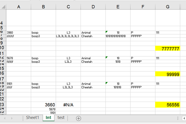
Is this even possible? I think it is, I really hope it is. I need to retrieve the highlighted amounts based off of a match. I have tried various index match formulas to no avail. My match will be the 4 digit id's in Col A. So if you look at B23, in C23 I want to retrieve G10's data. Then in B24 I will have the 5678 and I want to retrieve the next highlighted amount. Nothing is working for me. Here is the last formula I tried: =INDEX(A:G,4,7,MATCH(B23,A:A,0)). What am I doing wrong?

 

[Eric W]

You seem to have a few issues with your example. A6 is 3960, not 3660, and the 56556 values is 5 rows below A18, whereas G10 is 4 rows below A6, and G16 is 4 rows below A12. Assuming that's unintentional, try in C23:

=INDEX($H$10:$H$109,MATCH(B23,$A$6:$A$100,0))

Note the offset in rows, and make sure your ranges extend to the bottom of your data. If your sheet is not in a consistent format, it may be much tougher.

 

[Tash Point O]

Wow Eric,

That worked (I changed a few things on my sheet and your formula and it works)!! Would you be able to explain to me why I do not need to reference a row and column number for this and how this formula knows to go 4 rows down? Thank you so much for your help and no worries about answering the question, you've helped already.

You seem to have a few issues with your example. A6 is 3960, not 3660, and the 56556 values is 5 rows below A18, whereas G10 is 4 rows below A6, and G16 is 4 rows below A12. Assuming that's unintentional, try in C23:

=INDEX($H$10:$H$109,MATCH(B23,$A$6:$A$100,0))

Note the offset in rows, and make sure your ranges extend to the bottom of your data. If your sheet is not in a consistent format, it may be much tougher.

 

[Eric W]

It's an easy enough concept once you see it. The MATCH finds the matching location within the $A$6:$A$100 range, so if B23 is found in $A$6, MATCH returns a 1. Then the INDEX finds the value that is in the 1 position of $H$10:$H$109, which is H10. So the formula "knows" to go four rows down because the INDEX range starts 4 rows down from the MATCH range.

Glad to help!