
Running Totals
August 15, 2017 - by Bill Jelen

This episode shows three ways to do running totals.
A running total is, for a list of numeric values, a sum of the values from the first row to the row of the running total. Common uses of a running total are in a checkbook register or an accounting sheet. There are many ways to create a running total—two of which are described below.
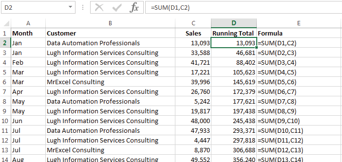
The simplest technique is to, on each row, add the running total from the row above to the value in the row. So the first formula in row 2 is:
=SUM(D1,C2)
The reason we use the SUM function is because, in the first row, we are looking at the header in the row above. If we use the simpler, more intuitive formula of =D1+C2 then an error will be generated because the header value is text versus numeric. The magic is that the SUM function ignores text values, which are added as zero values. When the formula is copied down to all of the rows in which a running total is desired, the cell references are adjusted accordingly:
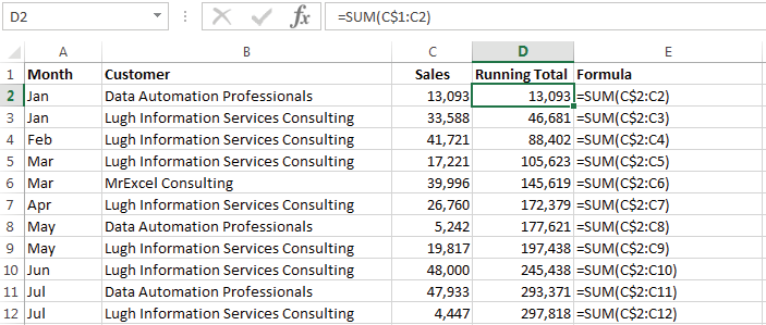
The other technique also uses the SUM function but each formula sums all of the values from the first row to the row displaying the running total. In this case we use a dollar sign ($) to make the first cell in the reference an absolute reference which means it is not adjusted when copied:
Both techniques are unaffected by sorting and deleting rows but, when inserting rows, the formula has to be copied into the new rows.
Excel 2007 introduced the Table which is a re-implementation of the List in Excel 2003. Tables introduced a number of very useful features for data tables such as formatting, sorting, and filtering. With the introduction of Tables we were also provided a new way of referencing the parts of a Table. This new referencing style is called structured referencing.
To convert the above example into a Table, we select the data we want to include in the Table and press Ctrl + T. After displaying a prompt asking us to confirm the Table's range and whether or not there are existing headers, Excel converts the data into a formatted Table:
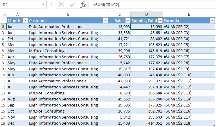
Note that the formulas we entered earlier remain the same.
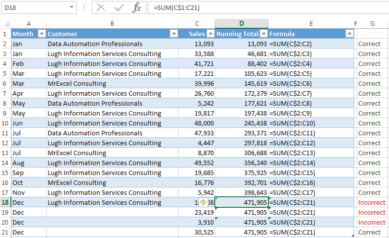
One of the useful features Tables offers is automatic formatting and formula maintenance as rows are added, removed, sorted, and filtered. It is the formula maintenance in particular that we will focus on and which can be problematic. To keep Tables working while they are manipulated, Excel utilizes calculated columns which are columns with formulas such as column D in the above example. When new rows are inserted are added to the bottom, Excel automatically populates the new rows with the “default” formula for that column. The problem with the above example is that Excel gets confused with standard formulas and does not always handle them correctly. This is made apparent when new rows are added to the bottom of the Table (by selecting the bottom right cell in the Table and pressing TAB):
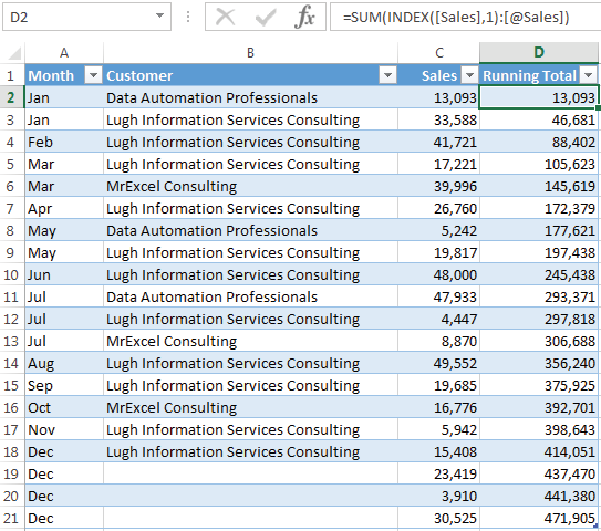
This deficiency is resolved by using the newer structured referencing. Structured referencing eliminates the need to reference specific cells using the A1 or R1C1 referencing style and instead uses column names and other keywords to identify and reference the parts of a Table. For example, to create the same running total formula used above but using structured referencing we have:
=SUM(INDEX([Sales],1):[@Sales])
In this example we have a reference to the column name, “Sales”, along with the at sign (@) to reference the row in the column in which the formula is located which is also known as the current row.
To implement the first example above where we added the running total value in the preceding row to the sales amount in the current row, you can use the OFFSET function:
=SUM(OFFSET([@[Running Total]],-1,0),[@Sales])
If the amounts used to calculate the running total are in two columns, for example one for “Debits” and one for “Credits”, then the formula is:
=SUM(INDEX( [Credit],1):[@Credit])- SUM(INDEX( [Debit],1):[@Debit])
Here we are using the INDEX function to locate the first row’s Credit and Debit cells, and summing the entire column up to and including the current row’s values. The running total is the sum of all credits up to and including the current row less the sum of all the debits up to and including the current row.

For a more information on structured references in particular and Tables in general, we recommend the book Excel Tables: A Complete Guide for Creating, Using and Automating Lists and Tables by Zack Barresse and Kevin Jones.
When I asked readers to vote for their favorite tips, tables were popular. Thanks to Peter Albert, Snorre Eikeland, Nancy Federice, Colin Michael, James E. Moede, Keyur Patel, and Paul Peton for suggesting this feature. Peter Albert wrote the Readable References bonus Tip. Zack Barresse wrote the Running Totals bonus tip. Four readers suggested using OFFSET to create expanding ranges for dynamic charts: Charley Baak, Don Knowles, Francis Logan, and Cecelia Rieb. Tables now do the same thing in most cases.
Watch Video
- This episode shows three ways to do running totals
- The first method has a different formula in Row 2 than all the other rows
- The first method is =Left in row 2 and =Left+Up in rows 3 through N
- If you try to use the same formula, you get a #Value error with =Total+Number
- Method 2 uses
=SUM(Up,Left)or=SUM(Previous Total,This Row Amount) - SUM ignores Text so you don't get a VALUE error
- Method 3 uses an expanding range:
=SUM(B$2:B2) - Expanding ranges are cool but they are slow
- Read the Charles Williams whitepaper on Excel Formula Speed
- The third method is a problem when you use Ctrl + T and add new rows
- Excel can't figure out how to write the formula
- The workarounds require some knowledge of structured referencing in Tables
- Workaround 1 is the slow
=SUM(INDEX([Qty],1):[@Qty]) - Workaround 2 is the volatile
=SUM(OFFSET([@Total],-1,0),[@Qty]) - [@Qty] refers to Qty on this row
- [Qty] refers to all Qty values
Video Transcript
Learn Excel for MrExcel Podcast, Episode 2004 -- Running Totals
I'll be podcasting this entire book. Click that I on the top right hand corner to subscribe.
Hey welcome back to the mystic cell netcast. I'm Bill Jelen. Now this topic in the book, I was contributed by my friend Zach Parise. Talk about Excel tables, Zach is the is the world's expert on Excel tables. He's written a book about Excel tables, but first let's talk about running totals not in tables.
So when I think about running totals, there's three different ways to do the running totals, and the way that I always started out with is in the first row you just say, bring the value over. So equal whatever's to the left of me. Alright so this format here is just =B2. These are all formula text here on the right-hand corner so you're seeing what we're using, and then from there on down, it's a simple little formula of equal the previous value, plus the current value right and copy that down, but you know now, we have this problem that it required two different formulas and you know in a perfect situation you have the exact same formula all the way down, and the reason we have to have a different formula there in the first row is that when you try and add equal 7 plus the word total it's a value error, but the cool worker out here, is to not just use left plus up, but to use =(SUM) of the previous value plus the quantity in this row, and see some is far enough to ignore texts. Right so that allows the same formula. all the way down.
Alright so that was when I was starting out using Excel, I was using that and then I discovered the expanding range, the expanding range says we're going to do L$2:L2 and what happens is this is always starting at row 2, but then it's going down to the current row. So when you look at how this works when it gets copied, we always started row 2, but we go down to the current row and this became my favorite method. I was like, oh, this is so much more sophisticated and when we go into Excel Options, go to the Formulas Tab and choose R1C1 in Reference Style. Alright see, R1C1, all of these formulas are exactly the same all the way down. I'm don't know if you understand R1C1, it's just good to know that we have identical R1C1 formulas all the way down.
Let's go back. So this method over here is the method that I liked, until until Charles Williams, an Excel MBP from England, who has an amazing paper on formula speed, Excel formula speed, completely debunked this method. This method, let's say you have 10,000 rows this, every single formula is looking at two references. So you're looking at 20,000 references, but this one, this is looking at two, this is looking at three, this is looking at four, this is looking at five and the last one is looking at 10,000 references, and it's horribly slower and so I stopped using this method.
Then I go on to read Zack in Kevin Jones's book about Excel tables and I discover yet another problem with this method. So one of the useful features the tables offers, is 'automatic formatting and formula maintenances rows are added, removed, sorted and filtered'. Alright that's a quote from his book. And to add a row to a table you just go to the very last cell on the table and press tab. So everything is working here. We're down to 70 right that's awesome and then A104 and I'll put in a 100 here. Alright, so that 70 should change to 170 and it does, but this 70 shouldn't have changed at all. Alright 68 + 2 is not a 170. I'll do it again. A 104 and put another hundred in the last one is right. These two are not right. Alright, so we have some weird situation that if you're using this formula and you convert over to table you start adding rows, the running total is not going to work. How bad is that?
Alright, so Zack offers two work arounds and both of them require a little bit of knowledge, of how structure references work. We're just going to have a new column out here and if I wanted to do quantity, equal quantity, right, so that =[@Qty] says quantity in this row. Oh cool, well there's another kind of reference where we use the Qty without the @. Check this out. So =SUM(INDEX([Qty),1:[@Qty]) means all of the quantities and we're going to say that we want to SUM from the first quantity, so (INDEX([Qty),1 says the first value here, down to the current row quantity, and this is using a really special version of index, when index is followed by a colon, it actually changes to a cell reference. Alright so, this workaround is unfortunately violating the Charles Williams rule of, we're going to have to look at every single reference, and so when you get 10,000 rows of this is going to go really, really slow.
Zach has another workaround that doesn't violate the Charles Williams problem, but it's using the dreaded OFFSET. OFFSET is a volatile function so every time that you calculate something, OFFSET is going to recalculate and everything down line from the OFFSET's going to recalculate. It's just a great way to completely, completely screw up your your formulas, and what this is doing, it's saying, we're taking the total from this row, going up one row, over zero columns and so what that's doing is saying: grab the total from the previous row and then we're adding to it the quantity from this row. Alright, so, now it's all looking at two references each time, but unfortunately the OFFSET is introducing volatile functions.
Well, there you have it, more than you ever wanted to know about Running Totals. I guess my final opinion here is to use this method, because it only looks it two. Same formula all the way down and your structured table references will work.
For this exploration and 39 other really good tips, check out this book MrExcel XL, the 40 greatest Excel tips of all time.
Recap for this episode we talked about three ways to do running totals. The first method has a different formula, row 2, than all the other rows. It's equal left in row 2 and then equal left plus up in rows 3 through N, but if you try and just use that same formula, equal left plus up, all the way down, how you're going to get a #Value Error. So =SUM(Up,Left), which is previous total, plus this roadmap, that works great, no Value Errors and then the expanding range which I use to love. They're cool, but until I read Charles Williams white paper on Excel form of speed. Then I started to hate these expanding references. It also has a problem when you use CTRL T and add new rows. Excel can't figure out how to expand that formula, how to add new rows. I love this tip go to the very last cell in the table and press Tab, that will add a new row and then we talked about some structured referencing, where we're using quantity in this row and then all quantities. =SUM(OFFSET([@Total],-1,00,[@Qty]).
Okay, I want thank Zach for contributing that tip. I want to thank you for stopping by. We'll see you next time for another netcast from MrExcel.
Download File
Download the sample file here: Podcast2004.xlsx
Title Photo: skeeze / pixabay