Change borders/gridlines of cells in rows A, B, C & D when cells in row E contains no blanks

David77

Board Regular
Joined
Jun 24, 2020
Messages
109
Office Version
  1. 365
Platform
  1. Windows
Hello everybody,

I am currently sitting with the following material overview file in Excel:


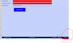
I have made some conditional formatting so whenever I enter a number in column E the entire row gets highlighted. Unfortunately, this erases/makes invisible my dark gridlines/borders from before. Naturally, I can (as you can see from the photo) create a conditional formatting for row E so whenever the value is not blank, it creates the dark gridline/border that I want (see the photo with the number 5 as an example).

However, I am not sure as to how I would go about with doing this for row A, B, C and D. Can somebody please help me with this?

P.S. I am not covering all of row A, B, C, D and E. It's only the values 36:495 for all of them in this list.

Thank you so much for your time everybody. I truly appreciate it!

Best regards,

David
 

Attachments

  • 1596716868653.png
    1596716868653.png
    52.2 KB · Views: 6

Excel Facts

Who is Mr Spreadsheet?
Author John Walkenbach was Mr Spreadsheet until his retirement in June 2019.
Hello. I tried solving your problem but I have one error, if it can be accepted on your side the formula is good to go. i.e. the error is the row which contains the number in E column will format the entire row with the same color as the row containing the header.
So the process is to select "new rule" under conditional formatting tab, and then select "use a formula to determine which cell to format", then define the rule as "=NOT(ISBLANK($E1))" then select border outline and also fill color.
Untitled2.jpg

Untitled.jpg

Book1
ABCDE
1NumberNameLocationcodeserial
245ankitindia788
340punitindia784
4785nehaindia781
5987rahulindia784
6452riyaindia7885
7456biswaindia741
82254abhiindia756
9789655sapnaindia742
1078522ranjitindia741
Sheet1
Cells with Conditional Formatting
CellConditionCell FormatStop If True
A1:E10Expression=NOT(ISBLANK($E1))textNO
 
Upvote 0
He
Hello. I tried solving your problem but I have one error, if it can be accepted on your side the formula is good to go. i.e. the error is the row which contains the number in E column will format the entire row with the same color as the row containing the header.
So the process is to select "new rule" under conditional formatting tab, and then select "use a formula to determine which cell to format", then define the rule as "=NOT(ISBLANK($E1))" then select border outline and also fill color.
View attachment 19805
View attachment 19806
Book1
ABCDE
1NumberNameLocationcodeserial
245ankitindia788
340punitindia784
4785nehaindia781
5987rahulindia784
6452riyaindia7885
7456biswaindia741
82254abhiindia756
9789655sapnaindia742
1078522ranjitindia741
Sheet1
Cells with Conditional Formatting
CellConditionCell FormatStop If True
A1:E10Expression=NOT(ISBLANK($E1))textNO
It worked!!!

Thank you so much! :) This is how I set it up btw (top one amongst the conditional formattings):

1596780213776.png


May I ask, if you have the spare time, would there be a way to augment the formula, so it does exactly the same as before, but also includes the formatting if the cell in row E is not blank AND not equal to 0 as well?

Thank you so much for your time!

Best regards,
David
 
Upvote 0
Hello, glad I could help. So if the E column contains number then the much easier way is to set "=$E>0", the formula gets the speed too in this case.
Book1
ABCDE
1NumberNameLocationcodeserial
245ankitindia7880
340punitindia784
4785nehaindia7815
5987rahulindia784
6452riyaindia7885
7456biswaindia741
82254abhiindia7560
9789655sapnaindia742
1078522ranjitindia741
Sheet1
Cells with Conditional Formatting
CellConditionCell FormatStop If True
A2:E10Expression=$E2>0textNO
 
Upvote 0

Forum statistics

Threads
1,215,050
Messages
6,122,868
Members
449,097
Latest member
dbomb1414

We've detected that you are using an adblocker.

We have a great community of people providing Excel help here, but the hosting costs are enormous. You can help keep this site running by allowing ads on MrExcel.com.
Allow Ads at MrExcel

Which adblocker are you using?

Disable AdBlock

Follow these easy steps to disable AdBlock

1)Click on the icon in the browser’s toolbar.
2)Click on the icon in the browser’s toolbar.
2)Click on the "Pause on this site" option.
Go back

Disable AdBlock Plus

Follow these easy steps to disable AdBlock Plus

1)Click on the icon in the browser’s toolbar.
2)Click on the toggle to disable it for "mrexcel.com".
Go back

Disable uBlock Origin

Follow these easy steps to disable uBlock Origin

1)Click on the icon in the browser’s toolbar.
2)Click on the "Power" button.
3)Click on the "Refresh" button.
Go back

Disable uBlock

Follow these easy steps to disable uBlock

1)Click on the icon in the browser’s toolbar.
2)Click on the "Power" button.
3)Click on the "Refresh" button.
Go back
Back
Top