Index/Match multiple hits of same cell value and add rows to fit spill

kidneythief

New Member
Joined
Mar 17, 2021
Messages
34
Office Version
  1. 365
Platform
  1. Windows
Hi guys! Not sure how to approach this - with lookup and aggregate, an index/match sub or something else.

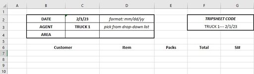
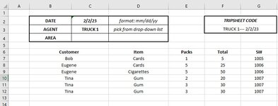
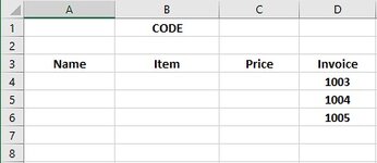
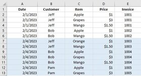
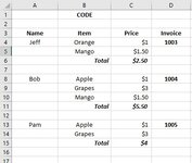
So In the sheet called Empty, when B2 is filled, it populates the Invoice column in D4:D with unique invoice numbers from an external order sheet.
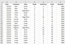
The Sales sheet has a list of orders where each invoice is broken down per item (so each single invoice number in the Empty sheet can have multiple instances
in the Sales sheet).

I need to pull data from the Sales sheet into the Empty sheet using the invoice numbers as a reference. However, since the Empty sheet only pulls a single
instance of each invoice number, I need to manage spillover and insert rows when needed, as seen in the Filled sheet.

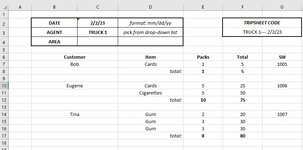
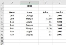
Going further, I was wondering if it would be possible to transpose output into something like what's shown in the Filled_Alt sheet, where Name and Invoice
(A2 and D2) are not repeated, and an extra row is added where the Price column items (or any additonal columns added there like quantity, etc.) are added up.

Ideally, the whole sheet would be populated as in Filled_Alt automatically each time B2 is changed and a new set of invoice numbers populate the D column.

Sorry to be asking so much, and I'd be really grateful for any help or guidance on this.
 

Attachments

  • Empty.jpg
    Empty.jpg
    18.9 KB · Views: 19
  • Filled.jpg
    Filled.jpg
    37.7 KB · Views: 21
  • Sales.jpg
    Sales.jpg
    63.3 KB · Views: 20
  • Filled_Alt.jpg
    Filled_Alt.jpg
    43.2 KB · Views: 19

Excel Facts

Who is Mr Spreadsheet?
Author John Walkenbach was Mr Spreadsheet until his retirement in June 2019.
Starting with the basic filled sheet, I've used a single sheet for simplicity in the example but it will work the same over multiple sheets.

If (as I'm assuming from the sample images) your criteria for the unique invoice numbers is the date then extracting them as unique is not necessary, it would be much simper to use the date criteria in the main formula in a single step. This may need some changes depending on how the results should be set out when there are multiple invoices with the same name. This particular layout would order the results by name rather than invoice number.

Kidneythief.xlsx
ABCDEFGHIJKL
1DateNameItemPriceInvoiceNameItemPriceInvoiceUnique
201/02/2023JeffApple11001JeffOrange110031003
301/02/2023JeffGrapes31001JeffMango1.510031004
401/02/2023JeffMango1.51001BobApple110041005
501/02/2023BobApple11002BobGrapes31004
601/02/2023BobMango1.51002BobMango1.51004
704/02/2023JeffOrange11003PamApple11005
804/02/2023JeffMango1.51003PamGrapes31005
904/02/2023BobApple11004
1004/02/2023BobGrapes31004
1104/02/2023BobMango1.51004
1204/02/2023PamApple11005
1304/02/2023PamGrapes31005
Sheet1
Cell Formulas
RangeFormula
G2:J8G2=FILTER(B2:E13,ISNUMBER(MATCH(E2:E13,L2#,0)))
L2:L4L2=UNIQUE(FILTER(E2:E13,A2:A13=DATE(2023,2,4)))
Dynamic array formulas.


The Filled_Alt sheet in your sample would not be possible with formulas. You could do something similar with a pivot table, although the resulting layout would not be exactly as your image.
The mini sheet below shows the output of a pivot table based on the original sales example, again the date is used as the criteria for the results to be returned.

Kidneythief.xlsx
ABCD
15Date04/02/2023
16
17NameInvoiceItemSum of Price
18Bob1004Apple$1.00
19Grapes$3.00
20Mango$1.50
211004 Total$5.50
22
23Bob Total$5.50
24
25Jeff1003Mango$1.50
26Orange$1.00
271003 Total$2.50
28
29Jeff Total$2.50
30
31Pam1005Apple$1.00
32Grapes$3.00
331005 Total$4.00
34
35Pam Total$4.00
Sheet1


Hope this helps.
 
Upvote 0
Hi, see the linked file (with 20 auxiliary columns) for a possible solution...
Wrong cells visible on Google Drive, because Google Drive does not know the LET function. All formulas work correctly with your Office 365.

The formulas used in the table:
tech!A2: =IF(OR(INDEX(Sales!A:A,ROW())="",INDEX(Sales!B:B,ROW())="",INDEX(Sales!E:E,ROW())=""),"",INDEX(Sales!A:A,ROW()))
tech!B2: =IF(OR(INDEX(Sales!A:A,ROW())="",INDEX(Sales!B:B,ROW())="",INDEX(Sales!E:E,ROW())=""),"",INDEX(Sales!B:B,ROW()))
tech!C2: =IF(OR(INDEX(Sales!A:A,ROW())="",INDEX(Sales!B:B,ROW())="",INDEX(Sales!E:E,ROW())=""),"",INDEX(Sales!C:C,ROW()))
tech!D2: =IF(OR(INDEX(Sales!A:A,ROW())="",INDEX(Sales!B:B,ROW())="",INDEX(Sales!E:E,ROW())=""),"",INDEX(Sales!D:D,ROW()))
tech!E2: =IF(OR(INDEX(Sales!A:A,ROW())="",INDEX(Sales!B:B,ROW())="",INDEX(Sales!E:E,ROW())=""),"",INDEX(Sales!E:E,ROW()))
tech!F2: =MAX(H:H)
tech!G2: =IF(A2="","",IF(COUNTIF(Empty!D:D,E2)>0,1,0))
tech!H2: =IF(A2="","",IF(G2=0,"",SUM(G$2:G2)+3))
tech!I2: =MAX(N:N)
tech!J2: =IF(A2="","",IF(G2=0,"",IF(E2=E1,"",1)))
tech!K2: =IF(A2="","",IF(G2=0,"",IF(E2=E1,"",IF(SUM(J$2:J2)=1,0,2))))
tech!L2: =IF(A2="","",IF(G2=0,"",SUM(G$2:G2)+SUM(K$2:K2)+3))
tech!M2: =IF(A2="","",IF(G2=0,"",IF(E2=E3,"",1)))
tech!N2: =IF(A2="","",IF(G2=0,"",IF(E2=E3,"",SUM(G$2:G2)+SUM(K$2:K2)+4)))
tech!O2: =IF(A2="","",IF(G2=0,"",IF(E2=E1,O1+D2,D2)))
tech!Q2: =IF(OR(INDEX(Orders!A:A,ROW())="",INDEX(Orders!B:B,ROW())=""),"",INDEX(Orders!A:A,ROW()))
tech!R2: =IF(OR(INDEX(Orders!A:A,ROW())="",INDEX(Orders!B:B,ROW())=""),"",INDEX(Orders!B:B,ROW()))
tech!S2: =MAX(U:U)
tech!T2: =IF(Q2="","",IF(Q2=Empty!B$1,1,0))
tech!U2: =IF(Q2="","",IF(T2=0,"",SUM(T$2:T2)+3))

Empty!D4: =IF(ROW()>tech!S$2,"",INDEX(tech!R:R,MATCH(ROW(),tech!U:U,0)))

Filled!A4: =IF(ROW()>tech!F$2,"",INDEX(tech!B:B,MATCH(ROW(),tech!H:H,0)))
Filled!B4: =IF(ROW()>tech!F$2,"",INDEX(tech!C:C,MATCH(ROW(),tech!H:H,0)))
Filled!C4: =IF(ROW()>tech!F$2,"",INDEX(tech!D:D,MATCH(ROW(),tech!H:H,0)))
Filled!D4: =IF(ROW()>tech!F$2,"",INDEX(tech!E:E,MATCH(ROW(),tech!H:H,0)))

Filled_Alt!A4: =LET(i,IFERROR(MATCH(ROW(),tech!L:L,0),0),IF(ROW()>tech!I$2,"",IF(i=0,"",IF(INDEX(tech!J:J,i)=1,INDEX(tech!B:B,i),""))))
Filled_Alt!B4: =LET(i,IFERROR(MATCH(ROW(),tech!L:L,0),0),j,IFERROR(MATCH(ROW(),tech!N:N,0),0),IF(ROW()>tech!I$2,"",IF(i=0,IF(j=0,"","Total"),INDEX(tech!C:C,i))))
Filled_Alt!C4: =LET(i,IFERROR(MATCH(ROW(),tech!L:L,0),0),j,IFERROR(MATCH(ROW(),tech!N:N,0),0),IF(ROW()>tech!I$2,"",IF(i=0,IF(j=0,"",INDEX(tech!O:O,j)),INDEX(tech!D:D,i))))
Filled_Alt!D4: =LET(i,IFERROR(MATCH(ROW(),tech!L:L,0),0),IF(ROW()>tech!I$2,"",IF(i=0,"",IF(INDEX(tech!J:J,i)=1,INDEX(tech!E:E,i),""))))

Multiple.xlsx
 
Upvote 0
Starting with the basic filled sheet, I've used a single sheet for simplicity in the example but it will work the same over multiple sheets.

If (as I'm assuming from the sample images) your criteria for the unique invoice numbers is the date then extracting them as unique is not necessary, it would be much simper to use the date criteria in the main formula in a single step. This may need some changes depending on how the results should be set out when there are multiple invoices with the same name. This particular layout would order the results by name rather than invoice number.

Kidneythief.xlsx
ABCDEFGHIJKL
1DateNameItemPriceInvoiceNameItemPriceInvoiceUnique
201/02/2023JeffApple11001JeffOrange110031003
301/02/2023JeffGrapes31001JeffMango1.510031004
401/02/2023JeffMango1.51001BobApple110041005
501/02/2023BobApple11002BobGrapes31004
601/02/2023BobMango1.51002BobMango1.51004
704/02/2023JeffOrange11003PamApple11005
804/02/2023JeffMango1.51003PamGrapes31005
904/02/2023BobApple11004
1004/02/2023BobGrapes31004
1104/02/2023BobMango1.51004
1204/02/2023PamApple11005
1304/02/2023PamGrapes31005
Sheet1
Cell Formulas
RangeFormula
G2:J8G2=FILTER(B2:E13,ISNUMBER(MATCH(E2:E13,L2#,0)))
L2:L4L2=UNIQUE(FILTER(E2:E13,A2:A13=DATE(2023,2,4)))
Dynamic array formulas.


The Filled_Alt sheet in your sample would not be possible with formulas. You could do something similar with a pivot table, although the resulting layout would not be exactly as your image.
The mini sheet below shows the output of a pivot table based on the original sales example, again the date is used as the criteria for the results to be returned.

Kidneythief.xlsx
ABCD
15Date04/02/2023
16
17NameInvoiceItemSum of Price
18Bob1004Apple$1.00
19Grapes$3.00
20Mango$1.50
211004 Total$5.50
22
23Bob Total$5.50
24
25Jeff1003Mango$1.50
26Orange$1.00
271003 Total$2.50
28
29Jeff Total$2.50
30
31Pam1005Apple$1.00
32Grapes$3.00
331005 Total$4.00
34
35Pam Total$4.00
Sheet1


Hope this helps.
Thank you for your replies! Whew, I think I'll need a day to go over these and process them!
Sorry if this omission made things confusing, but the contents of CODE are concatenated from a cell that indicates the date
and another cell that indicates a delivery truck number. The actual sheet where this will be applied has several sections of delivery orders
with headers in that exact format. So the goal was to have the data pulled depending on the indicated delivery truck number + the date.
Could I replace the Date function in the Unique/Filter formula with just the contents of a specified cell?
 
Last edited:
Upvote 0
Hi, see the linked file (with 20 auxiliary columns) for a possible solution...
Wrong cells visible on Google Drive, because Google Drive does not know the LET function. All formulas work correctly with your Office 365.

The formulas used in the table:
tech!A2: =IF(OR(INDEX(Sales!A:A,ROW())="",INDEX(Sales!B:B,ROW())="",INDEX(Sales!E:E,ROW())=""),"",INDEX(Sales!A:A,ROW()))
tech!B2: =IF(OR(INDEX(Sales!A:A,ROW())="",INDEX(Sales!B:B,ROW())="",INDEX(Sales!E:E,ROW())=""),"",INDEX(Sales!B:B,ROW()))
tech!C2: =IF(OR(INDEX(Sales!A:A,ROW())="",INDEX(Sales!B:B,ROW())="",INDEX(Sales!E:E,ROW())=""),"",INDEX(Sales!C:C,ROW()))
tech!D2: =IF(OR(INDEX(Sales!A:A,ROW())="",INDEX(Sales!B:B,ROW())="",INDEX(Sales!E:E,ROW())=""),"",INDEX(Sales!D:D,ROW()))
tech!E2: =IF(OR(INDEX(Sales!A:A,ROW())="",INDEX(Sales!B:B,ROW())="",INDEX(Sales!E:E,ROW())=""),"",INDEX(Sales!E:E,ROW()))
tech!F2: =MAX(H:H)
tech!G2: =IF(A2="","",IF(COUNTIF(Empty!D:D,E2)>0,1,0))
tech!H2: =IF(A2="","",IF(G2=0,"",SUM(G$2:G2)+3))
tech!I2: =MAX(N:N)
tech!J2: =IF(A2="","",IF(G2=0,"",IF(E2=E1,"",1)))
tech!K2: =IF(A2="","",IF(G2=0,"",IF(E2=E1,"",IF(SUM(J$2:J2)=1,0,2))))
tech!L2: =IF(A2="","",IF(G2=0,"",SUM(G$2:G2)+SUM(K$2:K2)+3))
tech!M2: =IF(A2="","",IF(G2=0,"",IF(E2=E3,"",1)))
tech!N2: =IF(A2="","",IF(G2=0,"",IF(E2=E3,"",SUM(G$2:G2)+SUM(K$2:K2)+4)))
tech!O2: =IF(A2="","",IF(G2=0,"",IF(E2=E1,O1+D2,D2)))
tech!Q2: =IF(OR(INDEX(Orders!A:A,ROW())="",INDEX(Orders!B:B,ROW())=""),"",INDEX(Orders!A:A,ROW()))
tech!R2: =IF(OR(INDEX(Orders!A:A,ROW())="",INDEX(Orders!B:B,ROW())=""),"",INDEX(Orders!B:B,ROW()))
tech!S2: =MAX(U:U)
tech!T2: =IF(Q2="","",IF(Q2=Empty!B$1,1,0))
tech!U2: =IF(Q2="","",IF(T2=0,"",SUM(T$2:T2)+3))

Empty!D4: =IF(ROW()>tech!S$2,"",INDEX(tech!R:R,MATCH(ROW(),tech!U:U,0)))

Filled!A4: =IF(ROW()>tech!F$2,"",INDEX(tech!B:B,MATCH(ROW(),tech!H:H,0)))
Filled!B4: =IF(ROW()>tech!F$2,"",INDEX(tech!C:C,MATCH(ROW(),tech!H:H,0)))
Filled!C4: =IF(ROW()>tech!F$2,"",INDEX(tech!D:D,MATCH(ROW(),tech!H:H,0)))
Filled!D4: =IF(ROW()>tech!F$2,"",INDEX(tech!E:E,MATCH(ROW(),tech!H:H,0)))

Filled_Alt!A4: =LET(i,IFERROR(MATCH(ROW(),tech!L:L,0),0),IF(ROW()>tech!I$2,"",IF(i=0,"",IF(INDEX(tech!J:J,i)=1,INDEX(tech!B:B,i),""))))
Filled_Alt!B4: =LET(i,IFERROR(MATCH(ROW(),tech!L:L,0),0),j,IFERROR(MATCH(ROW(),tech!N:N,0),0),IF(ROW()>tech!I$2,"",IF(i=0,IF(j=0,"","Total"),INDEX(tech!C:C,i))))
Filled_Alt!C4: =LET(i,IFERROR(MATCH(ROW(),tech!L:L,0),0),j,IFERROR(MATCH(ROW(),tech!N:N,0),0),IF(ROW()>tech!I$2,"",IF(i=0,IF(j=0,"",INDEX(tech!O:O,j)),INDEX(tech!D:D,i))))
Filled_Alt!D4: =LET(i,IFERROR(MATCH(ROW(),tech!L:L,0),0),IF(ROW()>tech!I$2,"",IF(i=0,"",IF(INDEX(tech!J:J,i)=1,INDEX(tech!E:E,i),""))))

Multiple.xlsx
Thank you fjns! Haha this is slightly overwhelming for me but I think I get the gist of it. So in your Orders sheet, I would have to list all invoice
numbers and assign a Code depending on the required grouping? The end-user I'm making this for may not be inclined to do much more than
fill in the date/delivery number so I'm trying to make their required effort to use the sheet be as little as possible 😅 But I think I learned quite
a bit from your formulas! I think I can use a bit of jasonb75 and your formulas to figure something out!
 
Upvote 0
I think I've muddied the question by attempting to simplify the source sheets too much so I'll repost with the actual sheet formats I'll be using.
Thank you though, I think your responses did technically give a solution considering the vague or missing information in the original post.
 
Upvote 0
Could I replace the Date function in the Unique/Filter formula with just the contents of a specified cell?
Going with the first method in my reply, I would suggest using just the first formula and replacing L2# with your original formula that you are using to extract the unique invoice numbers.

To get to the Alt layout, you would need to use the formula first, then create a pivot table similar to my second suggestion earlier from the table that the formula produces.

If you want to try it that way then I'll set up the example with instructions on how to create the pivot table.

Please be aware that I have a very unpredictable schedule over the next few days so may not be able to do this until the weekend. If you remove the solution flag from the post that you have marked then it is possible that someone else may pick up your thread and provide a solution sooner.
 
Upvote 0
I had a bit of time to look at this again. The mini sheet below takes information from the Sales and Orders sheets only, the Tech sheet is not needed for this.

Note that this is based on Office 365 as per your original question. Reading between the lines, there are things in your sample file that suggest a possible requirement for a google sheets formula. It is possible that the formula I have provided for you uses functions that will not work with google sheets.

MultipleNew.xlsx
ABCDEFGHI
1CODET0244949
2
3NameItemPriceInvoice
4JeffOrange11003NameInvoiceItemSum of Price
5JeffMango1.51003Bob1004Apple$1.00
6BobApple11004Grapes$3.00
7BobGrapes31004Mango$1.50
8BobMango1.510041004 Total$5.50
9PamApple11005
10PamGrapes31005Bob Total$5.50
11
12Jeff1003Mango$1.50
13Orange$1.00
141003 Total$2.50
15
16Jeff Total$2.50
17
18Pam1005Apple$1.00
19Grapes$3.00
201005 Total$4.00
21
22Pam Total$4.00
23
24Grand Total$12.00
25
Empty
Cell Formulas
RangeFormula
A4:D10A4=FILTER(Sales!B2:E30,ISNUMBER(MATCH(Sales!E2:E30,UNIQUE(FILTER(Orders!C2:C14,(LEFT(B1,3)=Orders!B2:B14)*(VALUE(RIGHT(B1,5))=Orders!A2:A14))),0)))
Dynamic array formulas.
 
Upvote 0
First of all, thank you for taking time to continue responding to my post! I really apologize for leaving some things out or kind of vague so I'll repost some of the details here.

In our actual distribution operations, we have 3 sales sheets, 4 delivery trucks, and daily sales/deliveries. The TripSheet is a record sent in by the delivery team, detailing which
orders (expressed as a single, consolidated invoice number) go in which truck on specific dates. We have 3 sales sheets covering 3 different suppliers with each unique item given
its own row, meaning a single invoice number in the TripSheet could have multiple entries of that same invoice number in the Sales sheets. The TripSheet and Sales sheets are
just sent to me in basically those formats. The end goal of the Output sheet is to be able to pull the invoice breakdowns based on both the DATE and also the TRUCK number. The
end user wants to use this as an overview when having trucks loaded prior to dispatching for delivery.

I have managed to pull data from and append the 3 sales sheets into this one Sales sheet which automatically updates when the source sales sheets are updated. The sales sheets,
unfortunately, do not indicate which trucks each order goes in, hence the need to get that information from the TripSheet, then match and expand the invoices as laid out in the
Sales sheets.

So what I have in the Output Sheet so far (and I'm not sure if it is the right approach), is 2 input fields for date and truck. I then have concat put those together as the Tripsheet Code
in F3. I then have a working sub pull only the invoices from Tripsheet with a matching Tripsheet Code. That leaves me with only the a single instance of each invoice in the Output
Sheet, so I need to somehow expand that to all the instances they appear in the sales sheets.

Alternatively, I was thinking it could be possible to add a column to the Sales sheet and pull what Truck they need to be loaded in based on the TripSheet? If I could do that then
maybe the combination UNIQUE/FILTER formulas would work that way?

Again, apologies for the unclear post but I hope this makes more sense now. Thank you!
 

Attachments

  • Output Sheet.jpg
    Output Sheet.jpg
    44.7 KB · Views: 9
  • OutputFilled.jpg
    OutputFilled.jpg
    67.1 KB · Views: 11
  • OutputFilledSums.jpg
    OutputFilledSums.jpg
    80 KB · Views: 7
  • Sales.jpg
    Sales.jpg
    105.6 KB · Views: 8
  • TripSheet.jpg
    TripSheet.jpg
    127.7 KB · Views: 9
Upvote 0

Forum statistics

Threads
1,215,328
Messages
6,124,299
Members
449,149
Latest member
mwdbActuary

We've detected that you are using an adblocker.

We have a great community of people providing Excel help here, but the hosting costs are enormous. You can help keep this site running by allowing ads on MrExcel.com.
Allow Ads at MrExcel

Which adblocker are you using?

Disable AdBlock

Follow these easy steps to disable AdBlock

1)Click on the icon in the browser’s toolbar.
2)Click on the icon in the browser’s toolbar.
2)Click on the "Pause on this site" option.
Go back

Disable AdBlock Plus

Follow these easy steps to disable AdBlock Plus

1)Click on the icon in the browser’s toolbar.
2)Click on the toggle to disable it for "mrexcel.com".
Go back

Disable uBlock Origin

Follow these easy steps to disable uBlock Origin

1)Click on the icon in the browser’s toolbar.
2)Click on the "Power" button.
3)Click on the "Refresh" button.
Go back

Disable uBlock

Follow these easy steps to disable uBlock

1)Click on the icon in the browser’s toolbar.
2)Click on the "Power" button.
3)Click on the "Refresh" button.
Go back
Back
Top