Creating a calendar by matching names and dates from multiple sheets

[mjreezy]

Hi, I am looking to create a calendar on the first tab of a workbook I have. Currently the workbook has multiple sheets of data, each sheet containing data related to a different type of work that is being scheduled in for different people. In order to currently find out what type of work someone is doing on any day they have to randomly click on each sheet tab and filter the data until they find their name on the date they are looking for, if its not on that tab sheet they have to repeat on each tab until they find it.
So I would like to have a formula that looks for the persons name in one cell, and date in another cell and finds the matching name and date on whichever sheet contains that name and date together, and returns the name of the sheet where that matching name and date is located. Ideally I would like it to return the name of the sheet where the matching name and date is as a hyperlink that when clicked on takes you to the row where the matching cell data was found. FYI, the names and dates are not in the same collumn on each sheet, one sheet the date and name could be in Collumn O & P, another sheet could be in J & F, but the name is always in the collumn to the right of the date on every sheet if that makes a difference.

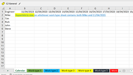
So by having this formula it should mean that someone only needs to look at the "Calendar" tab, which will be laid out with names in the Column A, and Dates in Row 1, to be able to see what type of work they are doing on any given day, and for more detail they can click on it and it will take them to the specific row on the sheet for that type of work where they can then view the other information contained on that sheet.

 

[excel_learnerz]

To achieve your goal, you can use a combination of functions like VLOOKUP, MATCH, and HYPERLINK in a formula to search for a matching name and date on each sheet in your workbook, and return the sheet name as a clickable hyperlink.

Here is an example formula that you can use in your calendar sheet:

=HYPERLINK("#'"&VLOOKUP($A2,INDIRECT("'"&$B$1&"'!$B:$B"),1,FALSE)&"'!A1","View Schedule")

This formula assumes that your calendar sheet has names in column A and dates in row 1, and that you have a cell (e.g. B1) where you enter the name of the sheet you want to search for a match.

The formula uses the VLOOKUP function to search for the name in column B of each sheet (specified by the sheet name in B1), and returns the corresponding sheet name using INDIRECT. It then uses HYPERLINK to create a clickable hyperlink that takes you to the first row of the matching name and date on the corresponding sheet.

You can copy and paste this formula to the cells in your calendar sheet for each name and date combination, and update the sheet name in B1 as needed.

Note that this formula assumes that each sheet has a consistent format where the name and date are always in the same columns, but in different columns across different sheets. If the column order is different for some sheets, you may need to adjust the formula accordingly.

 

[mjreezy]

To achieve your goal, you can use a combination of functions like VLOOKUP, MATCH, and HYPERLINK in a formula to search for a matching name and date on each sheet in your workbook, and return the sheet name as a clickable hyperlink.

Here is an example formula that you can use in your calendar sheet:

=HYPERLINK("#'"&VLOOKUP($A2,INDIRECT("'"&$B$1&"'!$B:$B"),1,FALSE)&"'!A1","View Schedule")

This formula assumes that your calendar sheet has names in column A and dates in row 1, and that you have a cell (e.g. B1) where you enter the name of the sheet you want to search for a match.

The formula uses the VLOOKUP function to search for the name in column B of each sheet (specified by the sheet name in B1), and returns the corresponding sheet name using INDIRECT. It then uses HYPERLINK to create a clickable hyperlink that takes you to the first row of the matching name and date on the corresponding sheet.

You can copy and paste this formula to the cells in your calendar sheet for each name and date combination, and update the sheet name in B1 as needed.

Note that this formula assumes that each sheet has a consistent format where the name and date are always in the same columns, but in different columns across different sheets. If the column order is different for some sheets, you may need to adjust the formula accordingly.

Hi, thank you very much for your response and formula that you suggested. However it doesn't work for my workbook. As mentioned I would like it to search across the entire workbook (all sheets) for the matching name and date, but I believe the above formula only will search a single sheet that I specify by entering a sheet name into a B1 cell, it won't search all the sheets from what I understand?.. Also my understanding is that the VLOOKUP is looking for names in collumn B, but on my workbook the names are on different collumns on each sheet e.g. on one sheet they are in collumn U and on another sheet they are in collumn J so I need it to be free to search every sheet and anywhere on every sheet.
From some research and using AI bot it looks like INDEX and maybe IFERROR would be the type of formula I need? But the AI bot ones are not working for me either yet!
Anything else you can suggest, or modifications to the formula above that would then fit in with what I am after?

Thank you so much again for taking your type to suggest the formula above, I very much appreciate it!
Mini sheets if it helps... I have dummed the workbook right down to the bare essentials to for testing purposes.

Calender work book test workbook for upload.xlsx
	A	B	C	D	E	F	G	H	I	J	K	L	M	N	O	P	Q
1		11/04/2023	12/04/2023	13/04/2023	14/04/2023	15/04/2023	16/04/2023	17/04/2023	18/04/2023	19/04/2023	20/04/2023	21/04/2023	22/04/2023	23/04/2023
2	Micheal Reed	Hyperlink to where there is a matching "Micheal Reed" and "11/04/2023".. Should return Work type 2 if it works correctly
3	Joe Bloggs		Hyperlink to where there is a matching "Joe Bloggs" and "12/04/2023".. Should return Work type 3 if it works correctly
4	John Dough			Hyperlink to where there is a matching "John Dough" and "13/04/2023".. Should return Work type 3 if it works correctly
5	Nick Ferry							Hyperlink to where there is a matching "Nick Ferry" and "17/04/2023".. Should return Work type 1 if it works correctly
Calendar

Thanks again, hopefully can help further

 

[mjreezy]

Hi, thank you very much for your response and formula that you suggested. However it doesn't work for my workbook. As mentioned I would like it to search across the entire workbook (all sheets) for the matching name and date, but I believe the above formula only will search a single sheet that I specify by entering a sheet name into a B1 cell, it won't search all the sheets from what I understand?.. Also my understanding is that the VLOOKUP is looking for names in collumn B, but on my workbook the names are on different collumns on each sheet e.g. on one sheet they are in collumn U and on another sheet they are in collumn J so I need it to be free to search every sheet and anywhere on every sheet.
From some research and using AI bot it looks like INDEX and maybe IFERROR would be the type of formula I need? But the AI bot ones are not working for me either yet!
Anything else you can suggest, or modifications to the formula above that would then fit in with what I am after?

Thank you so much again for taking your type to suggest the formula above, I very much appreciate it!
Mini sheets if it helps... I have dummed the workbook right down to the bare essentials to for testing purposes.

Calender work book test workbook for upload.xlsx
	A	B	C	D	E	F	G	H	I	J	K	L	M	N	O	P	Q
1		11/04/2023	12/04/2023	13/04/2023	14/04/2023	15/04/2023	16/04/2023	17/04/2023	18/04/2023	19/04/2023	20/04/2023	21/04/2023	22/04/2023	23/04/2023
2	Micheal Reed	Hyperlink to where there is a matching "Micheal Reed" and "11/04/2023".. Should return Work type 2 if it works correctly
3	Joe Bloggs		Hyperlink to where there is a matching "Joe Bloggs" and "12/04/2023".. Should return Work type 3 if it works correctly
4	John Dough			Hyperlink to where there is a matching "John Dough" and "13/04/2023".. Should return Work type 3 if it works correctly
5	Nick Ferry							Hyperlink to where there is a matching "Nick Ferry" and "17/04/2023".. Should return Work type 1 if it works correctly
Calendar

Thanks again, hopefully can help further

Hmm that mini sheet only was the first sheet of the workbook on it. Is there a way I can upload the workbook?

 

[Joe4]

Hmm that mini sheet only was the first sheet of the workbook on it. Is there a way I can upload the workbook?

No. You would have to upload it to a file sharing site and provide a link to it here.

 

[mjreezy]

Hi,

I have created a dummy copy of my workbook removing all but some data that would be enough to test out with formulas if that would help anyone with helping me with this.
On the first "Calendar" tab I have a few names and dates, which if the formula works in the highlighted yellow cells correctly, it should return a hyperlink of the name of one of the other sheets, that when clicked on takes you to the row where the matching name and date is located.

Workbook shared via toffeeshare:

Share files privately, fast and without size limit using ToffeeShare

Thank you in advance

 

[mjreezy]

Update... I am almost there... I have a formula that seems to work, sort of, its not returning the sheet name where the matching data is located but that's okay, instead it's displaying a message of "Click to see work" as a hyperlink which when clicked on takes me to the row where there is a match... BUT, the location where it is finding a match is just on the same sheet that the reference data used for the search is located in the first place! So I must need to alter the reference for the Named range that I am trying to get the formula to search in, so that it doesn't include the first "Calendar" sheet of my workbook.

This is the entire formula:
=HYPERLINK("#'"&INDEX(workbooksheets,MATCH(1,INDEX((workbooksheets<>"")*(COUNTIF(INDIRECT("'"&workbooksheets&"'!A:A"),$A4)>0)*(COUNTIF(INDIRECT("'"&workbooksheets&"'!1:1"),D$1)>0),),0))&"'!A"&MATCH($A4,INDIRECT("'"&INDEX(workbooksheets,MATCH(1,INDEX((workbooksheets<>"")*(COUNTIF(INDIRECT("'"&workbooksheets&"'!A:A"),$A4)>0)*(COUNTIF(INDIRECT("'"&workbooksheets&"'!1:1"),D$1)>0),),0))&"'!A:A"),0),"Click to see work")

The formula I have used to create the named range called "workbooksheets" is: "=GET.WORKBOOK(1) & T(NOW())" ... but obviously that means my formula will use that to search the whole workbook, but I don't want it it to search the first sheet!

I have tried this as well for another named range to use in the formula but formula doesn't work at all with this without success: ="'Work type 1'!$1:$1048576,'Work type 2'!$1:$1048576,'Work type 3'!$1:$1048576"

See Toffeeshare link to download my workbook with these latest attempts!

Share files privately, fast and without size limit using ToffeeShare

Send your files privately and fast. No file size limit. No registration. Peer to peer. End to end encrypted.

toffeeshare.com

Hopefully someone can help solve the last(hopefully) part of this puzzle!

Thank you